Technological Cell - Kinematic modeling
Kinematic modeling of manipulators plays an important role in contemporary robot control. It describes the relationship between robot end-effector position and orientation in space and manipulator joint angles. It also describes the correlation between linear and angular velocities of the end-effector and joint velocities.
The input of this part of the project is geometric model of the robot arms, we needed to make a kinematic model and then to make a program in C# so we can control the digital twin.
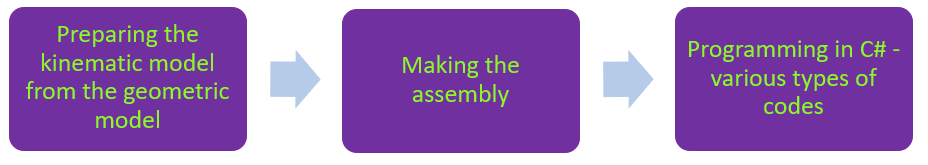
The first thing, that was done, was converting the geometric models of robots into kinematic models. To make a completely functional kinematic model we needed to disassemble the robot’s arms into the parts. The goal was to make an assembly from all the parts that need to be controlled and to add the environment (such as base, controlling systems, winding of wire…) as subassemblies. This is very important for the next stage, programming the control of robots.
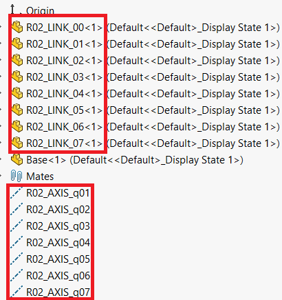
Then we renamed all the parts: R01_Link_00 (first part of the robot one- which is usually the base of the robot), R01_Link_01 (first part of the first robot), R02_Link_02 (third part of the second robot)… R01 or R02 defines the robot arm – R01 is for the robot welder and R02 is for the robot assistant. q is reserved for coincident or distance mates.
The mates between two parts (mates that define joints) should be concentric, coincidence, or distance. The coincident mate or distance mate needs to be between planes of both parts (for example mate between the right plane of the first part and the right plane of the second part is a coincidence). These kinds of mates we named R01_q01, R02_q01, R02_q02. Every part that defines one side of the joint needs to have its axis. These axes are also renamed: R01_AXIS_q01, R02_AXIS_q02…
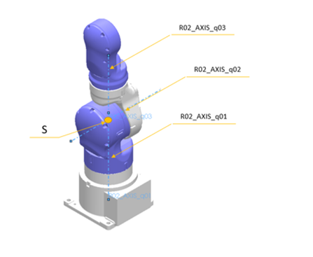
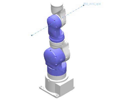
In the following picture, you can see the first three degrees of freedom and they all together create the shoulder joint. SIA10F is a perfect example of a copy of the human arm. The shoulder joint forms the structure of the spherical joint because the axes of these three parts are intersected at one point. That point is called S point, from the word shoulder. These three separate joints are revolute but when they are in the above-mentioned configuration, they all together make one spherical joint. This is very important for solving the inverse kinematics of the robot.
In the following picture is shown the fourth joint which has one degree of freedom – elbow.
The last three degrees of freedom are also projected so their axes are intersected in one point. This point is called W from the wrist. As at first three joints here also W point presents an integration of three revolute joints, each with one degree of freedom. This kind of joint is called the spherical joint.
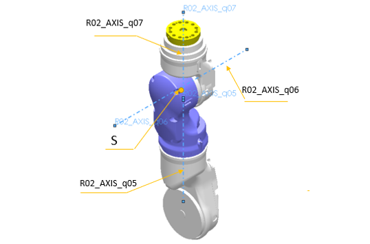
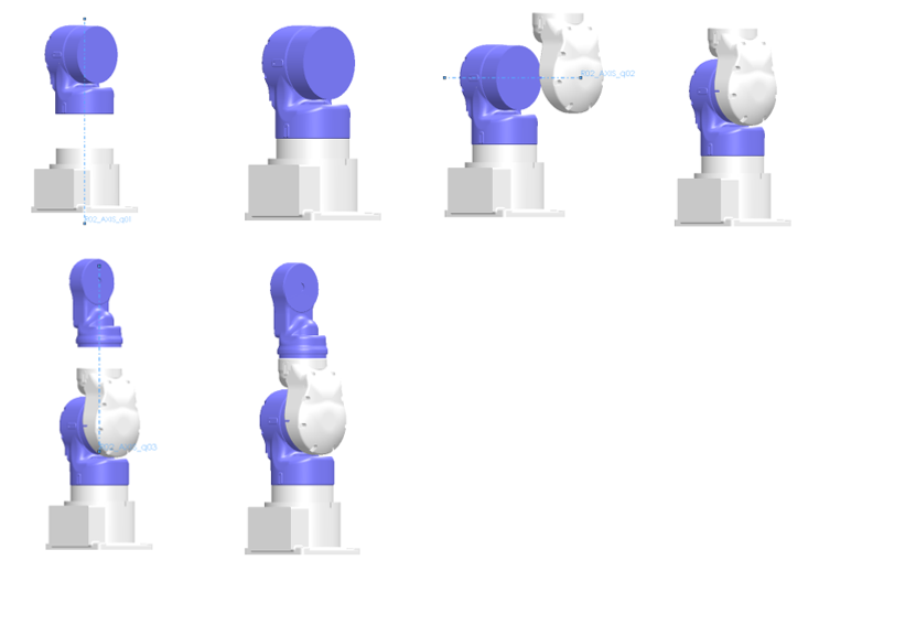
The architecture of this robot is interesting because it is designed as a human arm. The human arm has a spherical joint – shoulder in this robot it is represented as three separate revolute joints in which axes are intersected in one point, so they all together make one spherical joint. The fourth joint is a revolute joint, such as a human elbow it has just one degree of freedom. The rest of the joints also create a spherical joint in an above-mentioned way. In comparison to a human arm that is a wrist, which also has three degrees of freedom. The R-R-R-R-R-R-R kinematic architecture of the robot arm is converted in S-R-S (S from spherical and R from revolute). In the following pictures is shown how we made the assembly from the rest of the parts.
Problems, that we encountered in this part of the project, were merging all of the parts that define the joints correctly. We worked on downloaded 3D models of the robot’s arms. When we separated all the parts, we noticed that some surfaces which need to be circular, don’t have a regular circular shape. So, because of that, we couldn’t make the mates between two parts correctly. Therefore, the robot arm doesn’t have a full range of rotation around one joint, and this would represent a problem in the next stage when we control the robot arm with program code. Fortunately, our professor and assistant already had a model of SIA10F, that was made at our faculty. We proceeded to work with that one.
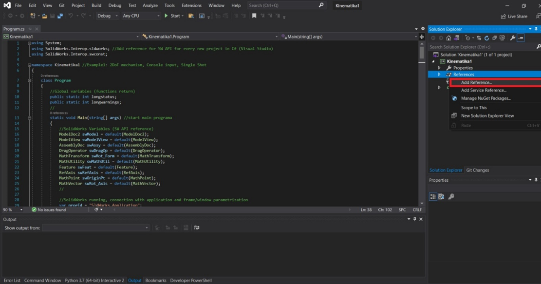
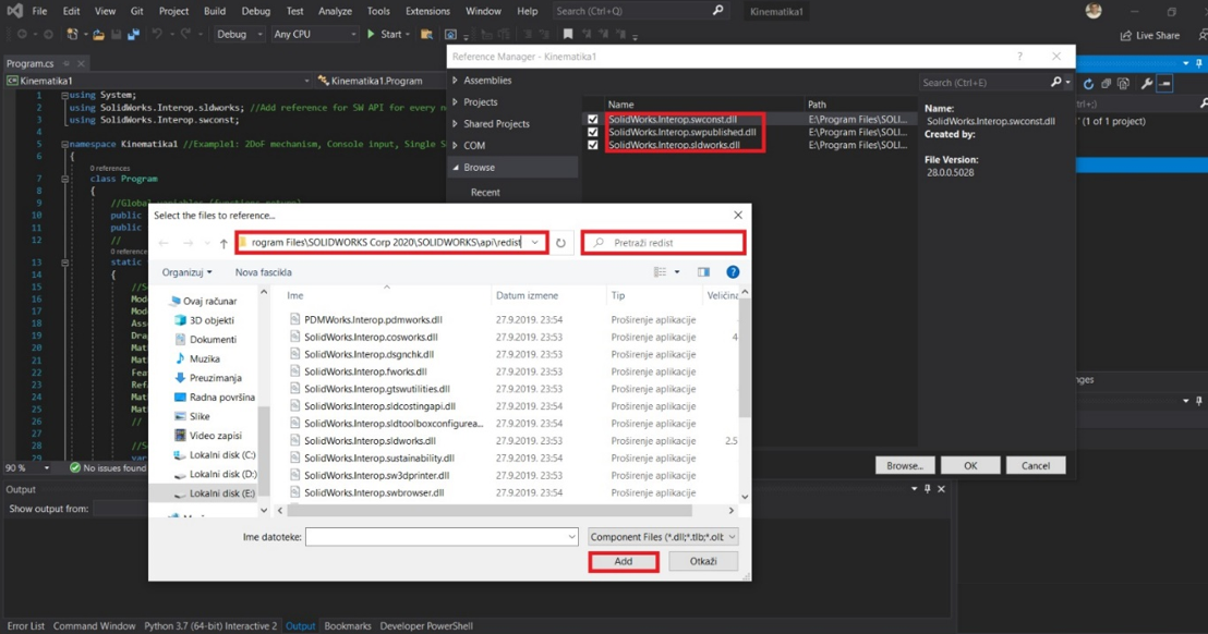
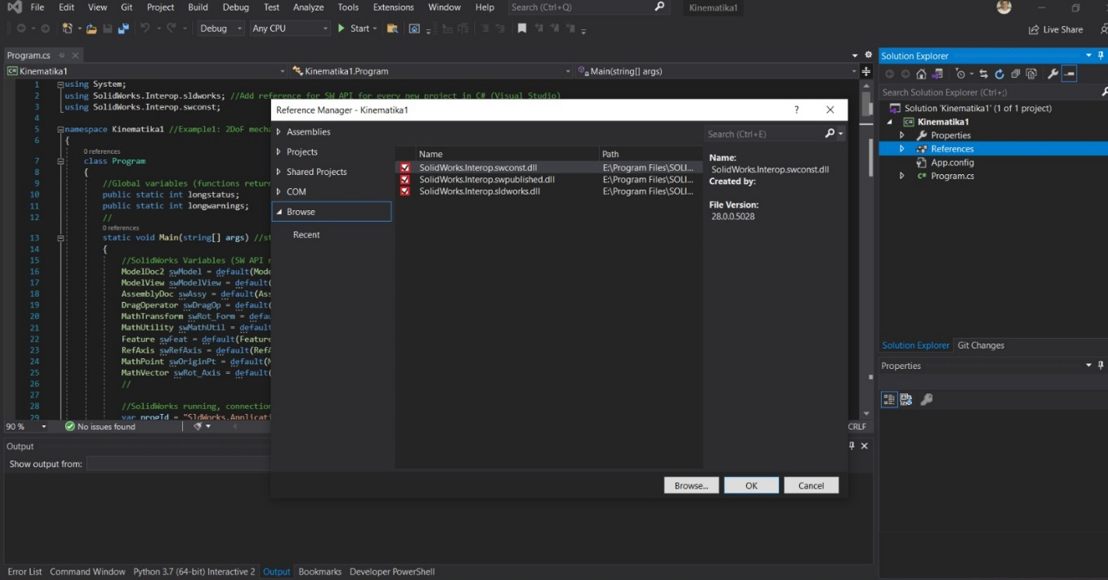
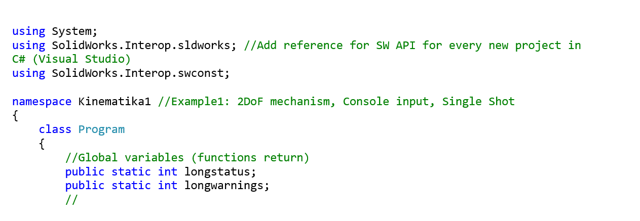
The next step was to make a program, which will execute the following task: We want to set the angles for every rotation or translation of the robot joints in command prompt, and the program needs to open the SW file and set these angles for each joint. The program for controlling of robot’s arms is made in Visual Studio C#. The following part of our report will be about explaining how this program works. The first step is about importing all the references that we will use in the program. They are related to SW API, in our case. At the right side of the C# should be the Solution Explorer, where References can be found. With the right click on the References appears drop-down menu. It is necessary to click on Add Reference, then to browse required references from the SolidWorks Corp folder, and then to add them to the project. This is shown in the following figures.
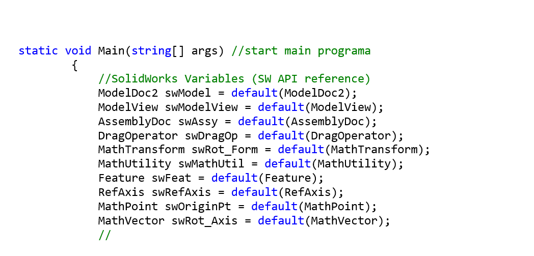
With the next step, we are defining all SolidWorks variables, which we are using. For example, we will use DragOperator for moving the robot’s arm from one point to another in SW, RefAxis will define an axis, around which part will rotate, MathTransform defines what will program execute whether rotation or translation…
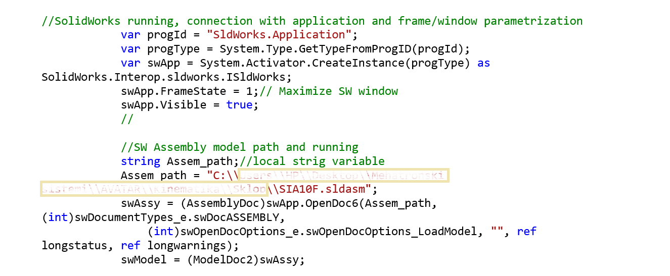
The following code lines are for opening the SW application and the assembly, in which we will operate. Here is very important to add the correct path of SW Assembly.
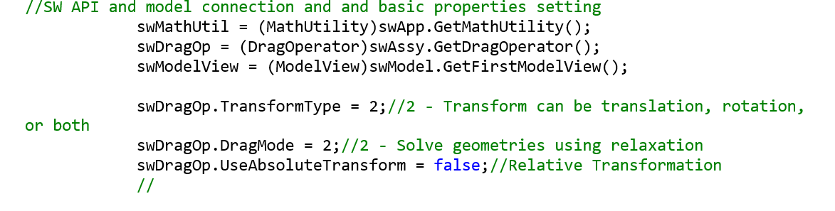
Then we need to connect SW API and model and to set basic properties with swDragOP.TransformType , we are defining transformation (0 is for translation 1 for rotation or 2 for both).
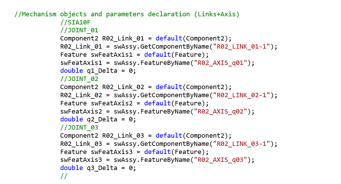
The next step is about defining the part that we will rotate, the reference axis, and the beginning angle of rotation. The next part of the program shows this for three parts of SIA10F. Here is important to set the same name of a part and an axis as in SW. By calling the parts from SW it is important to add the last number which defines which part is in the order with the same name (for example if there are two parts with the same name R01_Link_00 SolidWorks will add to the first of them suffix 1 and to the second suffix 2).
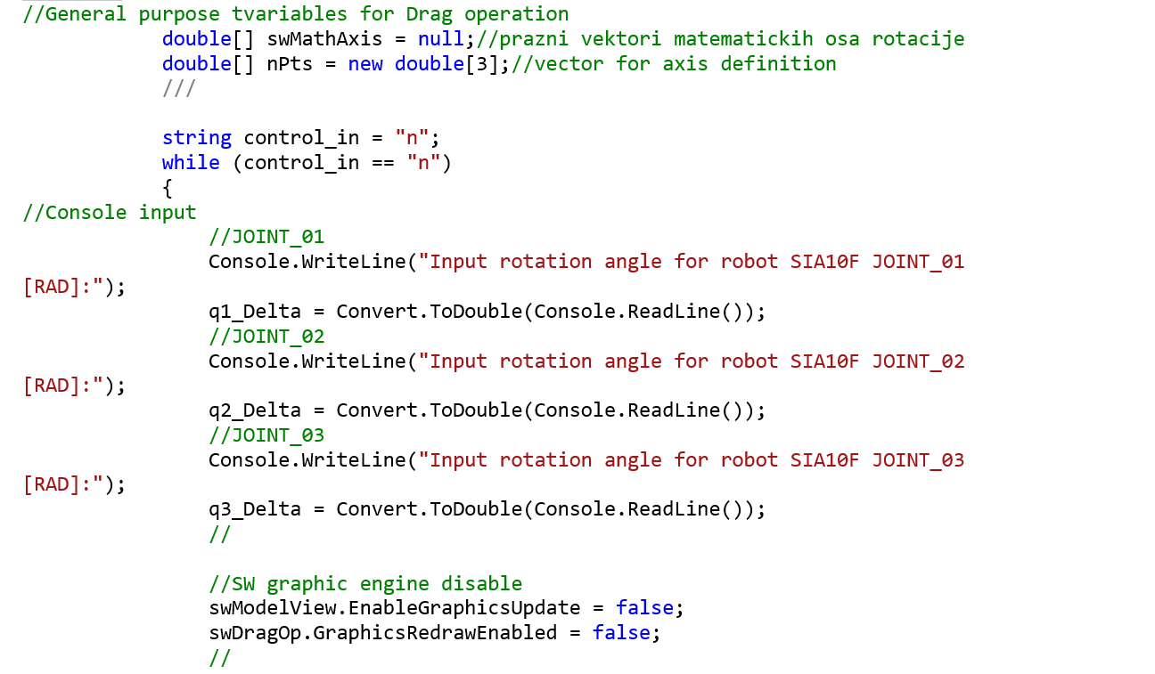
In the next step we need to read the angles from the console. That is shown in the following part of the program.
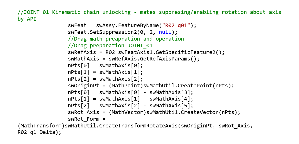
The next step is to prepare a drag operator. Before that we need to set a suppression of the mates. The idea is to suppress the mate that defines the angle between two parts, and with the drag operator to rotate or translate a part for the angle or distance entered in the console. With function swRefAxis.GetRefAxisParams we are reading the information (endpoint coordinates) for the currently selected reference axis.
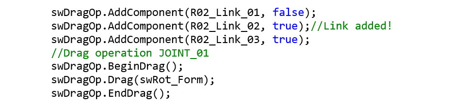
And with swDragOp.AddComponent is defined which part (link) will rotate or translate for a given angle or distance. false means that the selected part (in our case R02_Link_01) should rotate for a given angle, and true that selected parts (in our case R02_Link_02 and R02_Link_03) will follow R02_Link_01, without changing the angle between each other.
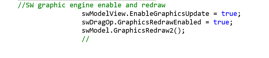
The last two parts of the code were shown only for one joint, the principle remains the same for other joints. The important thing is to define which part will move or rotate, and which parts will follow the movement, without changing the position between them. After all rotation and translation were defined, it is necessary to enable redrawing in SW, which is shown in the following part of the code.
The next step gives an option to set new angles or to exit the program.
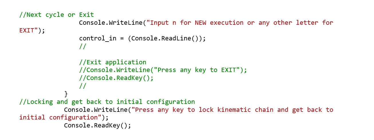
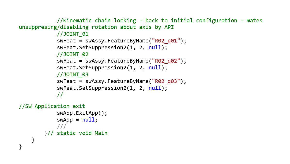
If it’s decided to exit SW, we are setting suppression back for all mates before closing the SW Application.
Script file generated in MATLAB environment
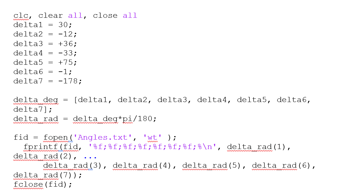
The following program executes entering the data (values) from MATLAB in the .txt file. This .txt file is read from C#. This code is just an example to show you that we can connect MATLAB and C#, which gives us a lot of possibilities. All the tools for calculations and data processing, that MATLAB possesses, can be used for connecting with the digital twin. First, we are defining all the angles of the robot arm and putting them in the vector. We need to create an empty .txt file in the same folder as this MATLAB Script. Then we are opening this .txt file from MATLAB with function fopen and writing the angles in it.
What is changed in C# code?
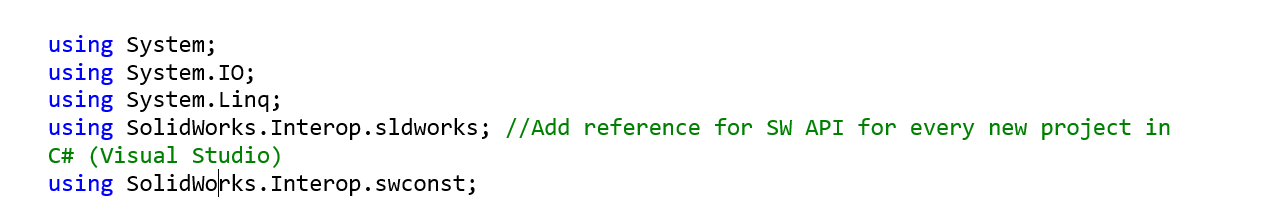
We are importing more references, which are shown in the following code lines.
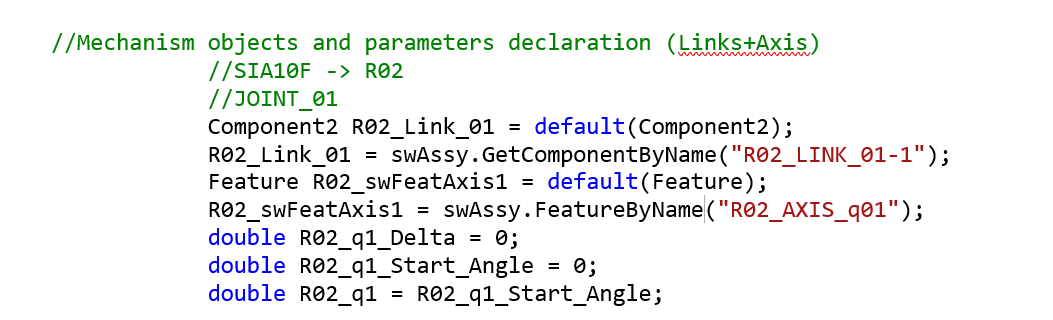
In the part when we are defining the features and the components, we are adding three new lines of the code (the last three lines). double R02_q1_Delta = 0 defines relative displacement angle, double R02_q1_Start_Angle = 0 defines start angle.
After that, we are loading .txt file and determining the length of lines and in the third part, we are determining the number of the columns.
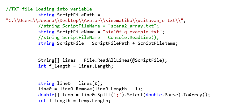
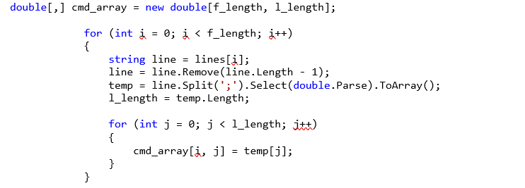
In the following lines of the code, we are defining for loop, for allocating the elements in the array.
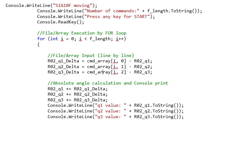
The next step is about starting up the program and calculation the absolute angle. The following part of the program is shown just for the first three angles, for the rest angles program code is similar.
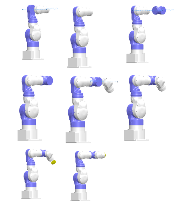
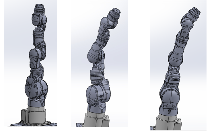
Problems that we had during programming were with mate suppressions. We thought that we should first suppress all the characteristics mates and then move parts, but that was not correct, because when we move the first part, other parts are not related with that part and they don’t move with the first part (after suppressing all the mates, all parts are independent between each other). So we came to the conclusion, that we need to suppress mate (just one mate, which defines observed joint), just before moving that part. For example, this problem is shown in the following three pictures. At the first picture is starting position of robot arm at the second is executed random moving of the robot, and at the third picture the robot should return to the starting position (the straight position). As you can see in this picture it makes some unfounded moves.
What did we learn?
The most important thing that we learned in this part of the project is CAD modeling at some higher level. By that, I mean transforming the geometric model into the kinetic model of the robot’s arm. Then we mastered the SolidWorks API library and we understood its advantages and disadvantages. Following that, we learned to read script file, which is generated from the MATLAB and in that way to control the robots. This makes a good base for the next step: connecting our 3D model with the real robot.
We have a great time during the Avatar project. We bring our knowledge on same higher levels, made new friendships, and learn something practical in our CMSysLab.